선행 지식 (Pre-requirement)
- RNN
- https://wikidocs.net/22886 - (딥러닝을 이용한 자연어 처리 입문)
- https://arxiv.org/abs/1808.03314 - (RNN paper)
- LSTM
- https://wikidocs.net/22888 - (딥러닝을 이용한 자연어 처리 입문)
- http://www.bioinf.jku.at/publications/older/2604.pdf - (LSTM paper)
- seq2seq model
- https://wikidocs.net/24996 - (딥러닝을 이용한 자연어 처리 입문)
- https://arxiv.org/abs/1409.3215 - (seq2seq paper)
"딥러닝을 이용한 자연어 처리 입문" 이라는 매우 좋은 책에 접근을 쉽게할 수 있는 만큼 많은 블로그에서 해당 문서를 토대로 적은 점을 확인했고, 본 포스트는 관련 논문을 토대로 작성하였으며 최대한 다양한 레퍼런스를 이용했습니다.

배경 (Background)
Bahdanau의 논문을 통해 attention이 등장하기 전까지는 neural machine translation(seq2seq)은 encoder-decoder RNN/LSTM 구조였다.
즉, 다음과 같은 단계를 거쳤다.
1. encoder LSTM은 모든 input sentence를 context vector로 변환
2. decoder LSTM or RNN units은 다음 단어를 생성
하지만 여기서의 문제는 long-range dependency problem이었는데, 이는 encoder가 안좋은 요약을 할 수록 translation은 안좋은 성능을 보인다는 점이며, 사실 문장의 길이 자체가 길 때 해당 문제가 발생하곤 했다.
LSTM이 사실 RNN의 고질적인 문제인 Long-range dependency를 거의 해결하긴 했으나 특정한 상황에서는 효과적이지 않은 경향이 있었다.
이때, Bahdanau는 다음과 같은 질문과 해결책을 제시함으로써 언급한 문제를 해결하고자 했다.
" 문장 내에서 서로 관련 있는 정보를 모두 유지할 순 없을까? " 라는 의문에서 시작.
"context vector 뿐만 아니라, 서로 관련있는 정보(relative importance) 도 각 Input words가 갖도록 해보자" 라는 해결책 제시
즉, 모델이 문장을 만들 때, encoder에서 가장 관련이 높은 정보를(the most relevant information) 확인할 수 있도록 하자.
* 해당 논문 (attention 등장 - 하지만 attention이라는 말을 직접적으로 사용하진 않았다)(Jointly Learning to Align이라는 말을 사용)
https://arxiv.org/abs/1409.0473
Neural Machine Translation by Jointly Learning to Align and Translate
Neural machine translation is a recently proposed approach to machine translation. Unlike the traditional statistical machine translation, the neural machine translation aims at building a single neural network that can be jointly tuned to maximize the tra
arxiv.org
Attention Mechanism
바로 본론으로 들어가겠다.

위의 그림에서 알 수 있다시피, Bidirectional LSTM은 annotation(h1,h2,...hT)(hidden state vector)을 generate하는데 사용된다.
기본적으로 각 X벡터는 encoder의 Hidden states 앞-뒤로 Concatenate되어 있다.

기존 encoder-decoder 모델에서는, encoder LSTM의 마지막 state만 context vector로써 사용했다.
하지만 위에서 언급한 바와 같이 context vector를 만들 때 모든 단어(words)의 embedding을 강조하며 hidden states의 weighted sum을 얻어내는 방법을 제안했다.
weighted sum을 계산하는 방법은 다음과 같다.


eij가 즉 feedforward neural network의 output score가 된다.

결국 a는 (Tx,1)차원의 벡터가 되고, element of a는 입력 문장에 해당하는 각 단어의 weights라고 볼 수 있다.
말과 이를 쉽게 해석해보면 다음과 같다.
" decoder에서 단어를 예측하는 모든 step마다 encoder의 input sequence를 이용하는 것, 이 때 encoder에서 가장 관련이 높은 정보를(the most relevant information) 확인할 수 있도록 하자 "
조금 더 깊게 들어가보자.
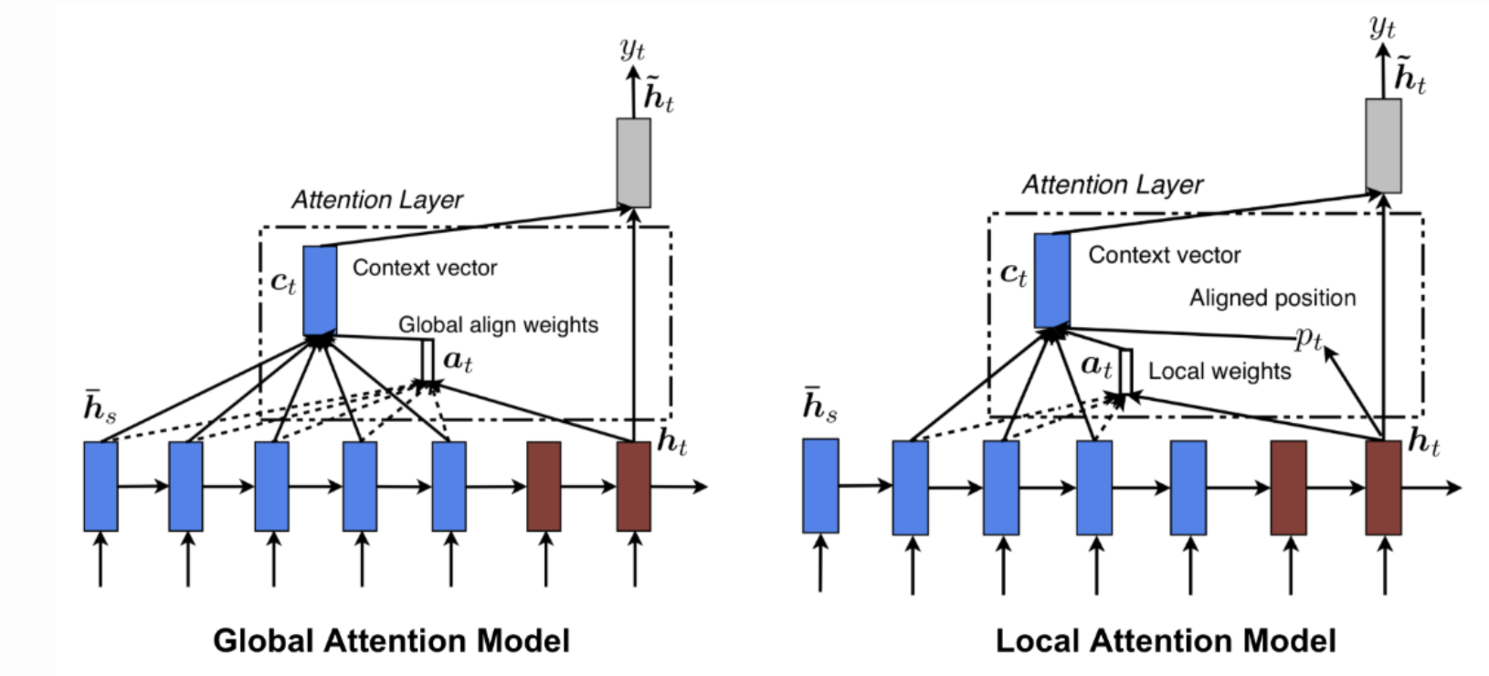
Global Attention vs Local Attention
Global Attention : 모든 input은 중요하다!
Luong, 2015, Effective Approaches to Attention-based Neural Machine Translation : https://arxiv.org/abs/1508.04025
Effective Approaches to Attention-based Neural Machine Translation
An attentional mechanism has lately been used to improve neural machine translation (NMT) by selectively focusing on parts of the source sentence during translation. However, there has been little work exploring useful architectures for attention-based NMT
arxiv.org
Global Attention 과 Bahdanau's Attention의 가장 큰 차이점은
Global attention은 "variable-length context vector"를 계산하기 위한 encoder LSTM과 decoder LSTM 모두의 hidden states를 모두 고려한다는 점, 반면 bahdanau's attention은 unidirecitonal decoder LSTM 그리고 encoder LSTM의 모든 hidden states를 사용하는 점이다.
사실, encoder-decoder architectures에서 score는 일반적으로 encoder의 function, decoder의 hidden states로 결정되는데 output word와 관계있는 input words의 relative importance를 찾을 수만 있다면 어떤 function을 쓰든 상관 없다.
따라서 Global Attention layer를 사용한다면 많은 양의 computation을 수반할 것이다. (모든 Hidden state가 고려 대상이 되기 때문에)
그렇다면 이때 양이 너무 큰것이 부담스러우니.. 나온 개념이 Local Attention이다.
이는 사실 soft and hard attention 의 컨셉에서 (vision task에서) 영감을 받은 것이다.
soft-hard는 ML에서 꽤나 자주 쓰이는 말로
soft: 모든 image patches가 일부 weight을 갖는 것이고,
hard: 하나의 image patch가 한 번에 고려되는 것
여기까지가 attention이 처음 등장한 때까지를 정리한 내용이며, 이제부터 많은 글들에서 나오는 key,query,value 개념이 나오는 transformers이다.
이때 key, query, values를 통해 attention을 일반적으로 재정의하게 된다.
Transformers - Attention is all you need
Transformers는 많은 사람들이 아는 architecture이다.
https://arxiv.org/abs/1706.03762
Attention Is All You Need
The dominant sequence transduction models are based on complex recurrent or convolutional neural networks in an encoder-decoder configuration. The best performing models also connect the encoder and decoder through an attention mechanism. We propose a new
arxiv.org
우선 "self-attention"이 무엇인지부터 정의하고 이어가보자.
LSTM이 나왔던 논문에서는 self-attention을 다음과 같이 정의한다.
The mechanism of relating different positions of a single sequence or sentence in order to gain a more vivid representation
직역하자면, 더 생생한(자연스러운-vivid) 표현을 위해 단일 시퀀스 혹은 문장의 서로 관련이 있으나 다른 위치들에 대한 체제이다.
위에서 문장에서 한 단어에 대한 attention을 계산하기 위해, score calculation의 mechanism은 dot production(내적)이나 이전에 봤던 단어들의 hidden states representation들로 어떤 특정한 function을 사용한다고 언급했었다.
하지만 지금 이 논문에서는 근본적으로는 같지만, 좀 더 일반적인 상황을 고려하여 개념을 제시한다.
The FBI is chasing a criminal on the run.
이라는 문장이 있다.
만약 "chasing"이라는 단어에 Attention을 계산한다고 가정해보자.
아마도 mechanism은 "chasing"에 대한 embedding 값을 "The", "FBI", "is"와 함께 dot production(내적)을 할 것이다.
이 상황을 일반화해서 적용시켜보자.
각 단어의 embedding은 서로 다른 세개의 벡터로 표현되는데 이때 우리는 이것을 Key, Query, Value 라고 부를 예정이다.
Query of target : input embedding과 관련된 attention을 계산하고자 할 때 사용
Key of the input : matching score를 계산할 때 사용
weights of the value vectors: summation시 사용
즉, Key, Query, Value는 각각 다른 subspaces의 embedding vector에 대한 abstractions일 뿐이다.
따라서 바로 위에서 말했던 예제에 일반화된 vector를 적용하면 Attention은 다음과 같다.
softmax(Q”chasing” . K”The” / D) : Query "chasing"에 대한 Key는 "The"이고 이때 value를 softmax function에 넣어준다.
softmax(Q”chasing” . K”FBI” / D) : so on
softmax(Q”chasing” . K”is” / D) : so on
즉 Q"target", K"input"으로 표현되는 하나의 함수일 뿐이다.
만약 벡터가 [0.2, 0.5, 0.3]의 값을 갖는다고 해보자.
이때 이 값들은 Attention의 계산을 위한 "alignment scores"가 되고, input embedding의 value vector와 곱해져서 weighted value vector를 구하고 이는 context vector를 얻는데 추가된다.
C”chasing”= 0.2 * VThe + 0.5* V”FBI” + 0.3 * V”is” (dot-production)
그리고 모든 embedding input vector는 하나의 matrix X에 combined되는데 다음과 같은 식을 가지게 된다.
Z=Softmax(Q*KT/D)V
만약 multi-headed Attention일 경우, matrix X는 서로 다른 K,Q,V를 얻기위해 서로다른 Wk, Wq, Wv matrices와 곱해진다.
즉, 3-headed self attention이라면 3개의 다른 Z matrices 또한 "Attention head"라고 칭하며 이때 이들은 모든 attention head에서 정보를 capture하기 위해 single attention head와 multiplication 및 concatenation을 한다.

밑의 도식은 참 유명한 transformers의 architecture다.

Multi-Head attention까지는 위에서 언급해서 이해가 되지만 Positional Encoding이 아직 무엇인지 설명을 안했으므로 이부분을 설명하겠다.
사실 지금까지 언급한 것들은 input words의 순서는 고려하지 않았다.
따라서 이를 capture하기 위해 positional encoding을 사용한다.
이 mechanism은 input embedding에 벡터를 추가하는데, 모든 벡터가 각 단어의 위치를 결정하는 것을 도와주거나 단어 사이의 거리를 찾는 것을 도와주는 특정한 턴을 따른다.
위의 그림 중 encoder부분을 간단히 설명하자면
첫째 sublayer에서는 multi-head self attention layer가 있고, additive residual connetion이 보인다. 그 위에 layer normalization layer가 존재하는데, 이는 batch normalization과 유사하다. (minibatch for calculation the normalization statistics)
그리고 같은 layer에 있는 모든 hidden units가 다시한번 계산되고 이에 대한 결과는 minibatch 위의 모든 neuron에 합해진 입력값이 된다. 그러므로 RNN/LSTM에 적용하기 편리하다.
두번째 sublayer에서는 feedforward layer가 있고, 모든 connection은 동일하다.
decoder부분에서는 encoder stack 맨 위에서부터 multi-head attention이 적용되는 layer가 있으며 모든 sublayer 이후 linear, softmax layer가 존재한다. 이렇게 output probabilities를 얻어낸다.
Attention을 위한 post이므로 masking 기법을 통한 prediction은 언급하지 않겠다.
참고 및 variants
https://www.youtube.com/watch?v=ycbMGyCPzvE
https://www.youtube.com/watch?v=rA28vBqN4RM
https://arxiv.org/abs/1409.3215
https://arxiv.org/abs/1409.0473
https://arxiv.org/abs/1601.06733
https://www.simplilearn.com/tutorials/deep-learning-tutorial/rnn
https://www.analyticsvidhya.com/blog/2019/11/comprehensive-guide-attention-mechanism-deep-learning/

'MACHINE LEARNING > Artificial Neural Network' 카테고리의 다른 글
| Sequence Modeling : Recurrent & Recursive Nets as RNN (0) | 2023.01.16 |
|---|---|
| Sequence Modeling : Recurrent & Recursive Nets as introduction (0) | 2023.01.15 |
| Few-Shot Learning? 관련 논문을 중심으로 이해해보자! (0) | 2022.12.27 |
| BART 논문 리뷰 / BART: Denoising Sequence-to-Sequence Pre-training for Natural Language Generation, Translation, and Comprehension (0) | 2022.11.28 |
| ML / Metric 종류 및 특징 정리 (0) | 2022.09.09 |